Introduction to the QuadratiK Package • QuadratiK

Overview

The QuadratiK package provides the first implementation, in R and Python, of a comprehensive set of goodness-of-fit tests and a clustering technique for spherical data using kernel-based quadratic distances. The primary goal of QuadratiK is to offer flexible tools for testing multivariate and high-dimensional data for uniformity, normality, comparing two or more samples.

This package includes several novel algorithms that are designed to handle spherical data, which is often encountered in fields like directional statistics, geospatial data analysis, and signal processing. In particular, it offers functions for clustering spherical data efficiently, for computing the density value and for generating random samples from a Poisson kernel-based density.

Installation

You can install the version published on CRAN of QuadratiK:

install.packages("QuadratiK")

Or the development version on GitHub:

library(devtools)
devtools::install_github('giovsaraceno/QuadratiK-package')

The QuadratiK package is also available in Python on PyPI and as a Dashboard application. Usage instruction for the Dashboard can be found at https://quadratik.readthedocs.io/en/latest/user_guide/dashboard_application_usage.html.

Citation

If you use this package in your research or work, please cite it as follows:

Saraceno G, Markatou M, Mukhopadhyay R, Golzy M (2024). QuadratiK: A Collection of Methods Constructed using Kernel-Based Quadratic Distances. https://cran.r-project.org/package=QuadratiK

@Manual{saraceno2024QuadratiK, 
   title = {QuadratiK: Collection of Methods Constructed using Kernel-Based 
            Quadratic Distances}, 
   author = {Giovanni Saraceno and Marianthi Markatou and Raktim Mukhopadhyay 
            and Mojgan Golzy}, 
   year = {2024}, 
   note = {<https://cran.r-project.org/package=QuadratiK>,
   <https://github.com/giovsaraceno/QuadratiK-package>, 
   <https://giovsaraceno.github.io/QuadratiK-package/>} 
}

and the associated paper:

Saraceno Giovanni, Markatou Marianthi, Mukhopadhyay Raktim, Golzy Mojgan (2024). Goodness-of-Fit and Clustering of Spherical Data: the QuadratiK package in R and Python. arXiv preprint arXiv:2402.02290.

@misc{saraceno2024package, 
   title={Goodness-of-Fit and Clustering of Spherical Data: the QuadratiK package in
          R and Python}, 
   author={Giovanni Saraceno and Marianthi Markatou and Raktim Mukhopadhyay and
           Mojgan Golzy}, 
   year={2024}, 
   eprint={2402.02290}, 
   archivePrefix={arXiv}, 
   primaryClass={stat.CO},    
   url={<https://arxiv.org/abs/2402.02290>}
}

Key features and basic usage

Goodness-of-Fit Tests

library(QuadratiK)

The software implements one, two, and k-sample tests for goodness of fit, offering an efficient and mathematically sound way to assess the fit of probability distributions. Our tests are particularly useful for large, high dimensional data sets where the assessment of fit of probability models is of interest.

The provided goodness-of-fit tests can be performed using the kb.test() function. The kernel-based quadratic distance tests are constructed using the normal kernel which depends on the tuning parameter \(h\). If a value for \(h\) is not provided, the function perform the select_h() algorithm searching for an optimal value. For more details please visit the relative help documentations.

?kb.test
?select_h

The proposed tests perform well in terms of level and power for contiguous alternatives, heavy tailed distributions and in higher dimensions.

Test for normality

To test the null hypothesis of normality \(H_0:F=\mathcal{N}_d(\mu, \Sigma)\)

x <- matrix(rnorm(100), ncol = 2)
# Does x come from a multivariate standard normal distribution?
kb.test(x, h=0.4)

## 
##  Kernel-based quadratic distance Normality test 
##      U-statistic V-statistic
## ------------------------------------------------
## Test Statistic:   1.719595    1.322694 
## Critical Value:   1.500279    8.901682 
## H0 is rejected:   TRUE        FALSE 
## Selected tuning parameter h:  0.4

If needed, we can specify \(\mu\) and \(\Sigma\), otherwise the standard normal distribution is considered.

x <- matrix(rnorm(100,4), ncol = 2)
# Does x come from the specified multivariate normal distribution?
kb.test(x, mu_hat = c(4,4), Sigma_hat = diag(2), h = 0.4)

## 
##  Kernel-based quadratic distance Normality test 
##      U-statistic V-statistic
## ------------------------------------------------
## Test Statistic:   -0.6502174      0.7549197 
## Critical Value:   1.999434    8.901682 
## H0 is rejected:   FALSE       FALSE 
## Selected tuning parameter h:  0.4

Two-sample test

In case we want to compare two samples \(X \sim F\) and \(Y \sim G\) with the null hypothesis \(H_0:F=G\) vs \(H_1:F\not =G\).

x <- matrix(rnorm(100), ncol = 2)
y <- matrix(rnorm(100,mean = 5), ncol = 2)
# Do x and y come from the same distribution?
kb.test(x, y, h = 0.4)

## 
##  Kernel-based quadratic distance two-sample test 
## U-statistic   Dn          Trace 
## ------------------------------------------------
## Test Statistic:   5.959489    10.47805 
## Critical Value:   0.7449454   1.311244 
## H0 is rejected:   TRUE        TRUE 
## CV method:  subsampling 
## Selected tuning parameter h:  0.4

k-sample test

In case we want to compare \(k\) samples, with \(k>2\), that is \(H_0:F_1=F_2=\ldots=F_k\) vs \(H_1:F_i\not =F_j\) for some \(i\not = j\).

x1 <- matrix(rnorm(100), ncol = 2)
x2 <- matrix(rnorm(100), ncol = 2)
x3 <- matrix(rnorm(100, mean = 5), ncol = 2)
y <- rep(c(1, 2, 3), each = 50)
# Do x1, x2 and x3 come from the same distribution?
x <- rbind(x1, x2, x3)
kb.test(x, y, h = 0.4)

## 
##  Kernel-based quadratic distance k-sample test 
## U-statistic   Dn          Trace 
## ------------------------------------------------
## Test Statistic:   7.934695    11.82316 
## Critical Value:   0.8798716   1.312038 
## H0 is rejected:   TRUE        TRUE 
## CV method:  subsampling 
## Selected tuning parameter h:  0.4

Test for uniformity on the sphere

Expanded capabilities include supporting tests for uniformity on the d-dimensional Sphere based on Poisson kernel. The Poisson kernel depends on the concentration parameter \(\rho\) and a location vector \(\mu\). For more details please visit the help documentation of the pk.test() function.

?pk.test

To test the null hypothesis of uniformity on the \(d\)-dimensional sphere \(\mathcal{S}^{d-1} = \{x \in \mathbb{R}^d : ||x||=1 \}\)

# Generate points on the sphere from the uniform ditribution 
x <- sample_hypersphere(d = 3, n_points = 100)
# Does x come from the uniform distribution on the sphere?
pk.test(x, rho = 0.7)

## 
##  Poisson Kernel-based quadratic distance test of 
##                         Uniformity on the Sphere 
## Selected consentration parameter rho:  0.7 
## 
## U-statistic:
## 
## H0 is rejected:  FALSE 
## Statistic Un:  -0.6928069 
## Critical value:  2.019198 
## 
## V-statistic:
## 
## H0 is rejected:  FALSE 
## Statistic Vn:  15.76902 
## Critical value:  23.22949

Poisson kernel-based distribution (PKBD)

The package offers functions for computing the density value and for generating random samples from a PKBD. The Poisson kernel-based densities are based on the normalized Poisson kernel and are defined on the \(d\)-dimensional unit sphere. For more details please visit the help documentation of the dpkb() and rpkb() functions.

?dpkb
?rpkb

Example

mu <- c(1,0,0)
rho <- 0.9
x <- rpkb(n = 100, mu = mu, rho = rho)
head(x$x)

##           [,1]        [,2]         [,3]
## [1,] 0.9780912 -0.08471612  0.190159960
## [2,] 0.9997680 -0.02148703 -0.001506489
## [3,] 0.9987756 -0.03309853 -0.036767684
## [4,] 0.9543338  0.29842370  0.013791345
## [5,] 0.9972640  0.05695963 -0.047117547
## [6,] 0.9892089 -0.14298927 -0.031933722

dens_x <- dpkb(x$x, mu = mu, rho = rho)
head(dens_x)

##            [,1]
## [1,]  1.3755632
## [2,] 14.2197297
## [3,] 11.2147895
## [4,]  0.5400748
## [5,]  8.2924525
## [6,]  2.9956620

Clustering Algorithm for Spherical Data

The package incorporates a unique clustering algorithm specifically tailored for spherical data and it is especially useful in the presence of noise in the data and the presence of non-negligible overlap between clusters. This algorithm leverages a mixture of Poisson kernel-based densities on the Sphere, enabling effective clustering of spherical data or data that has been spherically transformed. For more details please visit the help documentation of the pkbc() function.

?pkbc

Example

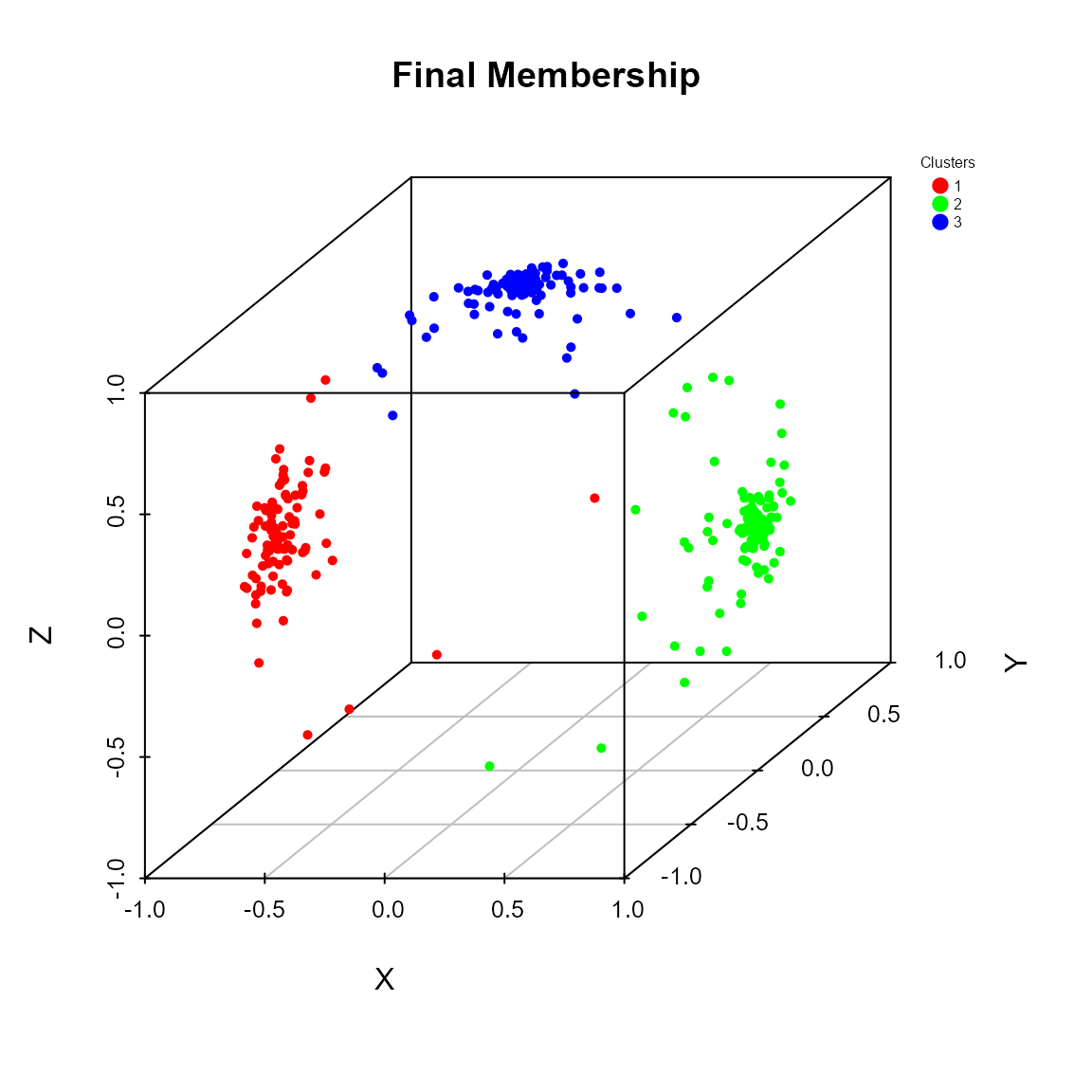
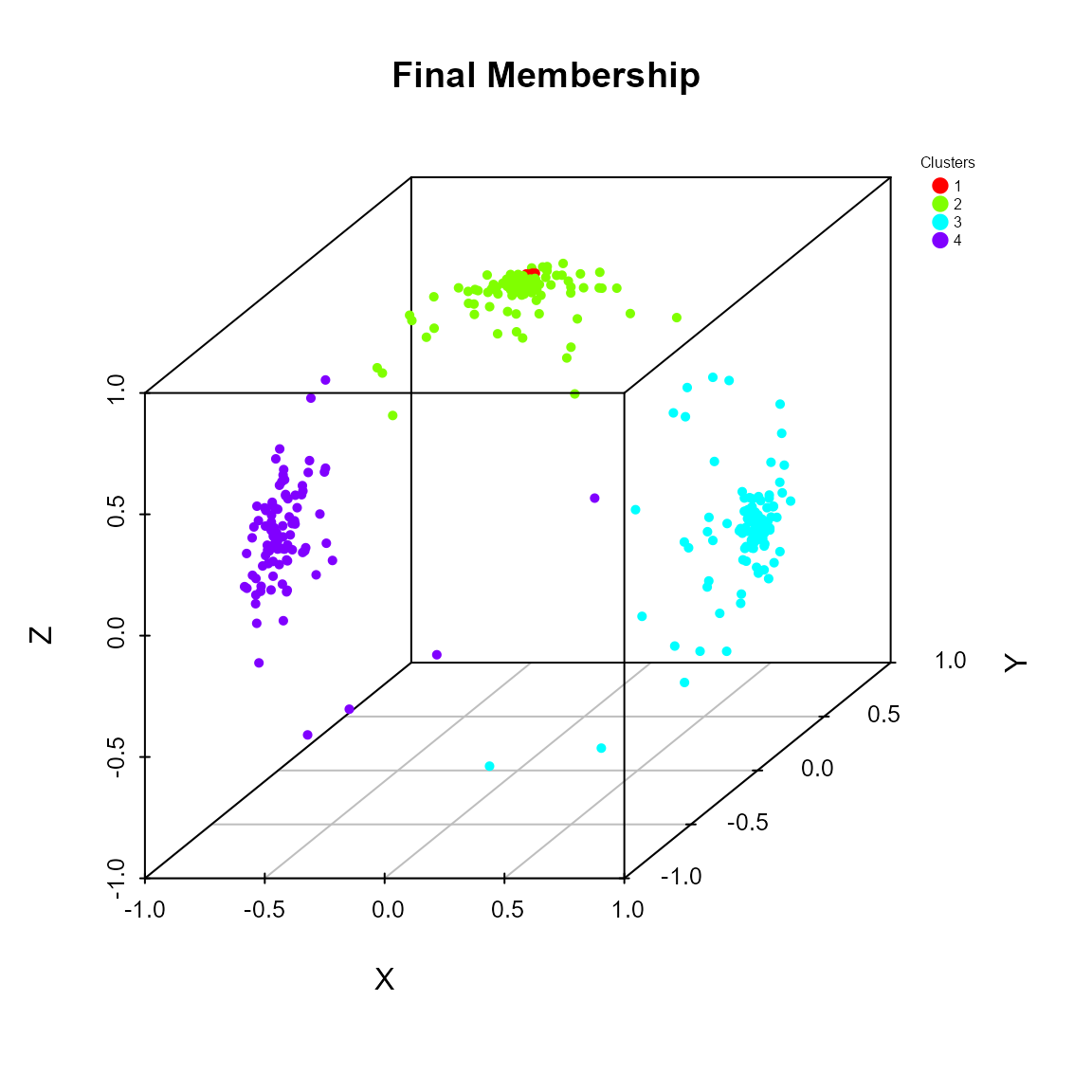
# Generate 3 samples from the PKBD with different location directions
x1 <- rpkb(n = 100, mu = c(1,0,0), rho = rho)
x2 <- rpkb(n = 100, mu = c(-1,0,0), rho = rho)
x3 <- rpkb(n = 100, mu = c(0,0,1), rho = rho)
x <- rbind(x1$x, x2$x, x3$x)
# Perform the clustering algorithm
# Serch for 2, 3 or 4 clusters
cluster_res <- pkbc(dat = x, nClust = c(2, 3, 4))
summary(cluster_res)

## Poisson Kernel-Based Clustering on the Sphere (pkbc) Results
## ------------------------------------------------------------
## 
## Summary:
##         LogLik     WCSS
## [1,] -590.5130 411.9053
## [2,] -236.2047 314.8386
## [3,] -229.8145 314.7841
## 
## Results for 2 clusters:
## Estimated Mixing Proportions (alpha):
## [1] 0.3000705 0.6999295
## 
## Clustering table:
## 
##   1   2 
##  89 211 
## 
## 
## Results for 3 clusters:
## Estimated Mixing Proportions (alpha):
## [1] 0.3288503 0.3318632 0.3392865
## 
## Clustering table:
## 
##   1   2   3 
##  98 102 100 
## 
## 
## Results for 4 clusters:
## Estimated Mixing Proportions (alpha):
## [1] 0.02161394 0.31559674 0.33298479 0.32980453
## 
## Clustering table:
## 
##   1   2   3   4 
##   5  95 102  98

The software includes additional graphical functions, aiding users in validating and representing the cluster results as well as enhancing the interpretability and usability of the analysis.

# Predict the membership of new data with respect to the clustering results
x_new <- rpkb(n = 10, mu = c(1,0,0), rho = rho)
memb_mew <- predict(cluster_res, k = 3, newdata = x_new$x)
memb_mew$Memb

##  [1] 2 2 2 2 2 2 2 2 2 2

# Compute measures for evaluating the clustering results
val_res <- pkbc_validation(cluster_res)
val_res

## $metrics
##             2         3         4
## ASW 0.5148733 0.7415262 0.4223992
## 
## $IGP
## $IGP[[1]]
## NULL
## 
## $IGP[[2]]
## [1] 1 1
## 
## $IGP[[3]]
## [1] 1 1 1
## 
## $IGP[[4]]
## [1] 1 1 1 1

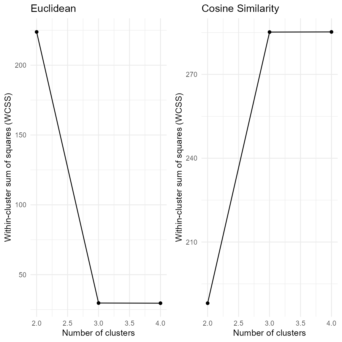
# Plot method for the pkbc object:
# - scatter plot of data points on the sphere
# - elbow plot for helping the choice of the number of clusters
plot(cluster_res)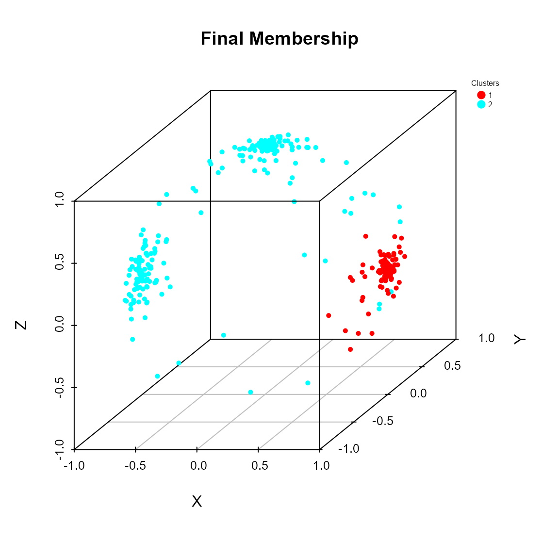

Additional Resources

For more detailed information about the QuadratiK package, you can explore the following resources:

Package Documentation on CRAN – Official package documentation on CRAN.
GitHub Repository – The GitHub repository with the development version, issues, and community discussions.
QuadratiK Package Website – A dedicated website with additional tutorials and examples.

If you’re new to the package, we recommend starting with the available vignettes:

References

For more information on the methods implemented in this package, refer to the associated research papers:

Markatou, M. and Saraceno, G. (2024). “A Unified Framework for Multivariate Two- and k-Sample Kernel-based Quadratic Distance Goodness-of-Fit Tests.” arXiv:2407.16374
Ding, Y., Markatou, M. and Saraceno, G. (2023). “Poisson Kernel-Based Tests for Uniformity on the d-Dimensional Sphere.” Statistica Sinica. doi: 10.5705/ss.202022.0347.
Golzy, M. and Markatou, M. (2020) Poisson Kernel-Based Clustering on the Sphere: Convergence Properties, Identifiability, and a Method of Sampling, Journal of Computational and Graphical Statistics, 29:4, 758-770, DOI: 10.1080/10618600.2020.1740713.