Clustering algorithm on the Wireless data
Source:vignettes/wireless_clustering.Rmd
wireless_clustering.RmdThe Wireless Indoor Localization Data
We consider the Wireless Indoor Localization Data Set, publicly
available in the UCI Machine Learning Repository’s website. This data
set is used to study the performance of different indoor localization
algorithms. It is available within the QuadratiK package as
wireless.
##    V1  V2  V3  V4  V5  V6  V7 V8
## 1 -64 -56 -61 -66 -71 -82 -81  1
## 2 -68 -57 -61 -65 -71 -85 -85  1
## 3 -63 -60 -60 -67 -76 -85 -84  1
## 4 -61 -60 -68 -62 -77 -90 -80  1
## 5 -63 -65 -60 -63 -77 -81 -87  1
## 6 -64 -55 -63 -66 -76 -88 -83  1
The Wireless Indoor Localization data set contains the measurements of the Wi-Fi signal strength in different indoor rooms. It consists of a data frame with 2000 rows and 8 columns. The first 7 variables report the values of the Wi-Fi signal strength received from 7 different Wi-Fi routers in an office location in Pittsburgh (USA). The last column indicates the class labels, from 1 to 4, indicating the different rooms. Notice that, the Wi-Fi signal strength is measured in dBm, decibel milliwatts, which is expressed as a negative value ranging from -100 to 0. In total, we have 500 observations for each room.
In many wireless applications, the relative signal strengths across routers are more relevant to the underlying spatial patterns and device positioning than the absolute magnitudes. Additionally, absolute signal strength can be affected by noise, device orientation or environmental factors. In this case, it is reasonable to consider the spherically transformed data points using L2 normalization. This transformation maps the data onto the surface of a 6-dimensional sphere, ensuring that each observation has a uniform length. Given that absolute signal strength is not critical to the research question, the spherical representation provides a meaningful and interpretable framework for studying the data set. In general, it is appropriate to consider spherically transformed data points when: (i) the absolute length of the measurements is irrelevant or too noisy; (ii) if we are more interested in the relative distributions (or angular relationships) between data points.
We perform the clustering algorithm on the wireless data
set. We consider the \(K= 3, 4, 5\) as
possible values for the number of clusters.
wire <- wireless[,-8]
labels <- wireless[,8]
wire_norm <- wire/sqrt(rowSums(wire^2))
set.seed(2468)
res_pk <- pkbc(as.matrix(wire_norm),3:5)
The pkbc function creates an object of class
pkbc containing the clustering results for each value of
number of clusters considered.
To guide the choice of the number of clusters, the function
pkbc_validation provides cluster validation measures and
graphical tools. Specifically, it returns an object with InGroup
Proportion (IGP), and metrics, a table of computed
evaluation measures. This table includes the Average Silhouette Width
(ASW) and, if the true labels are provided, the measures of adjusted
rand index (ARI), Macro-Precision and Macro-Recall.
set.seed(2468)
res_validation <- pkbc_validation(res_pk, true_label = labels)
res_validation$IGP
## [[1]]
## NULL
##
## [[2]]
## NULL
##
## [[3]]
## [1] 0.9860558 0.9706215 0.9429038
##
## [[4]]
## [1] 0.9662698 0.9733607 0.9526627 0.9880240
##
## [[5]]
## [1] 0.9713701 0.7727273 0.9880240 0.9639831 0.9433498
round(res_validation$metrics, 5)## 3 4 5
## ASW 0.35326 0.38031 0.30240
## ARI 0.69526 0.94031 0.91409
## Macro_Precision 0.18389 0.97719 0.00120
## Macro_Recall 0.26000 0.97700 0.00150The clusters identified with \(k=4\) achieve high values of ARI, Macro Precision and Macro Recall.
For a brief description of the reported evaluation measures, with the
corresponding references, please visit the help documentation of the
pkbc_validation function.
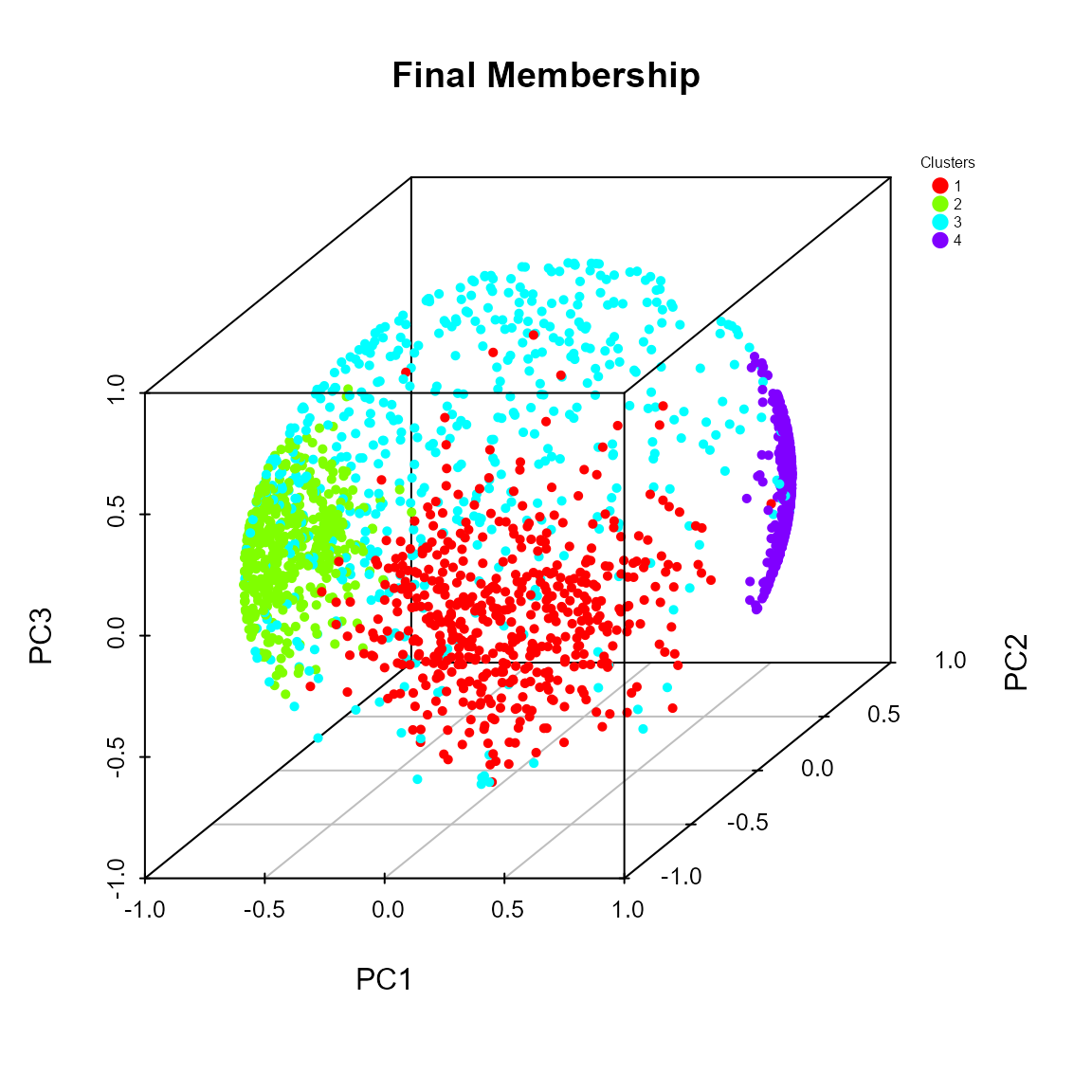
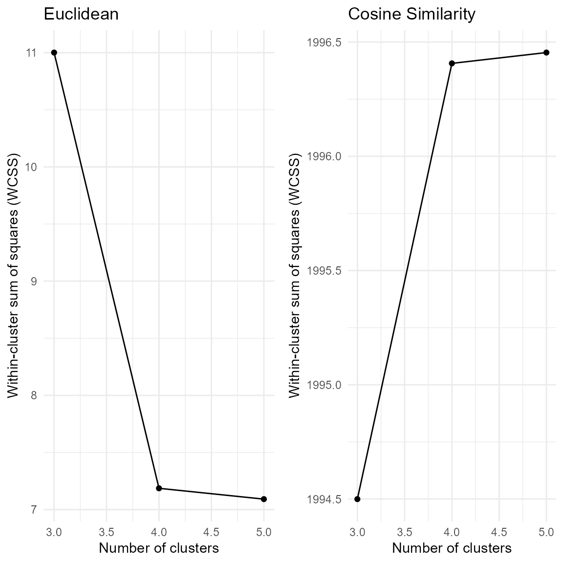
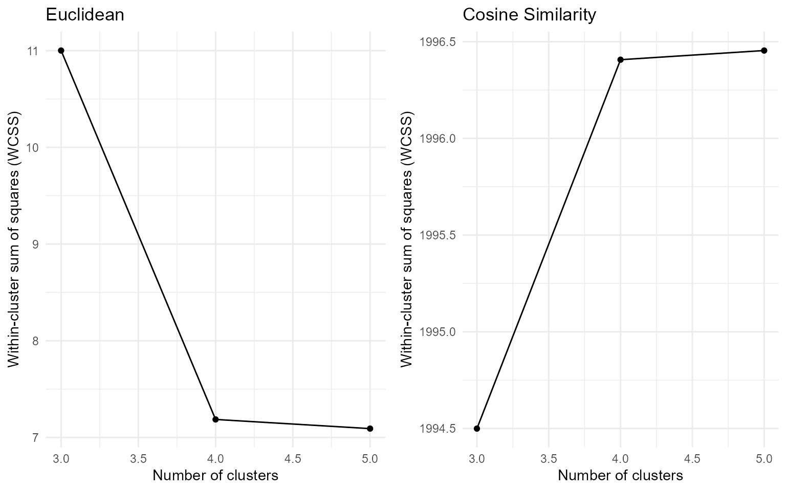
help(pkbc_validation)The plot method of the pkbc class can be
used to display the scatter plot of data points and the Elbow plot from
the computed within-cluster sum of squares values. For the scatter plot,
for \(d=2\) and \(d=3\), observations are displayed on the
unit circle and unit sphere, respectively. If \(d>3\), the spherical PCA is applied on
the data set, and the first 3 principal components are used for
visualizing data points on the sphere. In the generated scatter plot for
the specified number of clusters, data points are colored by the
assigned membership.
plot(res_pk, k = 4)

The Elbow plots and the reported metrics suggest \(K=4\) as number of clusters. This is in accordance with the known ground truth.
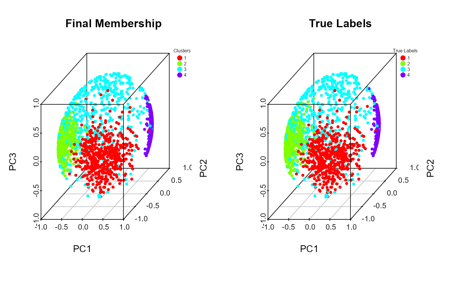
Additionally, if true labels are available and are provided to the
plot method, the scatter plot will display the data points
colored with respect to the true labels and assigned memberships in two
adjacent plots.
plot(res_pk, k=4, true_label = labels)

The plot of points using the principal components also shows that the identified cluster follows the initial labels.
Once the number of clusters is selected, the method
summary_stat can be used to obtain additional summary
information with respect to the clustering results. In particular, the
function provides mean, standard deviation, median, inter-quantile
range, minimum and maximum computed for each variable, overall and by
the assigned membership.
summary_clust <- stats_clusters(res_pk,4)
summary_clust## [[1]]
## Group 1 Group 2 Group 3 Group 4 Overall
## mean -0.33976246 -0.23423419 -0.29470203 -0.34377323 -0.30363137
## sd 0.01283014 0.05324085 0.01581506 0.01298448 0.05251967
## median -0.33952107 -0.24604104 -0.29625176 -0.34242063 -0.31847692
## IQR 0.01674475 0.03014941 0.02182651 0.01835030 0.06412536
## min -0.37455424 -0.30643954 -0.34994496 -0.39357081 -0.39357081
## max -0.29339739 -0.06308050 -0.23847076 -0.31226867 -0.06308050
##
## [[2]]
## Group 1 Group 2 Group 3 Group 4 Overall
## mean -0.30636324 -0.35918738 -0.32636022 -0.31540450 -0.32655905
## sd 0.01392354 0.02052666 0.01842337 0.01608549 0.02635941
## median -0.30600005 -0.35809184 -0.32487137 -0.31538238 -0.32221067
## IQR 0.01958541 0.02460137 0.02426854 0.02263003 0.03624468
## min -0.35600342 -0.45578394 -0.40026324 -0.36631517 -0.45578394
## max -0.26903743 -0.30605235 -0.27775661 -0.27586207 -0.26903743
##
## [[3]]
## Group 1 Group 2 Group 3 Group 4 Overall
## mean -0.32905221 -0.35786158 -0.31417147 -0.28929074 -0.32231793
## sd 0.01563476 0.02459888 0.01710971 0.02094437 0.03163402
## median -0.32915518 -0.35575396 -0.31237754 -0.29072716 -0.32209343
## IQR 0.01957377 0.03437142 0.02422092 0.02851547 0.03973413
## min -0.38248214 -0.43623816 -0.38676345 -0.33639128 -0.43623816
## max -0.28256746 -0.28237524 -0.26460827 -0.23485570 -0.23485570
##
## [[4]]
## Group 1 Group 2 Group 3 Group 4 Overall
## mean -0.34918727 -0.24111635 -0.30079691 -0.35013402 -0.31082318
## sd 0.01475930 0.04839750 0.01973759 0.01679759 0.05251032
## median -0.34858664 -0.24898566 -0.30107248 -0.35004522 -0.32519736
## IQR 0.01898212 0.03356955 0.02672633 0.02286452 0.06907237
## min -0.40129910 -0.31690470 -0.35542814 -0.41273961 -0.41273961
## max -0.30779911 -0.07399736 -0.23119131 -0.30906423 -0.07399736
##
## [[5]]
## Group 1 Group 2 Group 3 Group 4 Overall
## mean -0.38226045 -0.43319403 -0.37583631 -0.28257085 -0.36807675
## sd 0.01770626 0.02787579 0.01814674 0.02110273 0.05820777
## median -0.37991233 -0.43009295 -0.37549563 -0.28337199 -0.37738801
## IQR 0.02531565 0.04108696 0.02541214 0.02710382 0.06966093
## min -0.45385132 -0.52580164 -0.42808192 -0.34353824 -0.52580164
## max -0.34027255 -0.36916034 -0.33333333 -0.21464345 -0.21464345
##
## [[6]]
## Group 1 Group 2 Group 3 Group 4 Overall
## mean -0.45125600 -0.46327257 -0.48366352 -0.49713921 -0.47391075
## sd 0.01446455 0.02195263 0.01814601 0.01412842 0.02488735
## median -0.45081811 -0.46519225 -0.48319020 -0.49649227 -0.47411000
## IQR 0.01833254 0.02770315 0.02503768 0.01895624 0.03825696
## min -0.51475369 -0.53938031 -0.53130759 -0.53840040 -0.53938031
## max -0.41652096 -0.40313011 -0.44107352 -0.45551482 -0.40313011
##
## [[7]]
## Group 1 Group 2 Group 3 Group 4 Overall
## mean -0.45728346 -0.46863418 -0.48984740 -0.49701329 -0.47827795
## sd 0.01710219 0.02396734 0.01993870 0.01587742 0.02515570
## median -0.45703017 -0.46920446 -0.49013407 -0.49711582 -0.47914650
## IQR 0.02311965 0.03050579 0.02784124 0.02030659 0.03643335
## min -0.50728615 -0.56835661 -0.54571977 -0.53648350 -0.56835661
## max -0.41326597 -0.38995633 -0.43815927 -0.44423198 -0.38995633Note
If the number of cluster k is not provided to the
plot function, one scatter plot is displayed for each
possible number of clusters available in the object of class
pkbc.
References
Golzy, M. and Markatou, M. (2020). “Poisson Kernel-Based Clustering on the Sphere: Convergence Properties, Identifiability, and a Method of Sampling,” Journal of Computational and Graphical Statistics, 29(4), 758-770. DOI: 10.1080/10618600.2020.1740713.